2.10. Programming: Assistance in selected tasks

Learn to program code without AI writing code

Subject: Programming  ·  Grade: 9 (age 14–15)  ·  Duration: 1 double lesson (90 min) ·  AI: Assistance WITH AI 

AI-related competencies (DUAL.AI.TEACHer Framework) – teacher level

Subject-specific learning objectives – student/learner level

AF-TL-2b (AI foundations and applications × Teaching & Learning, Level 2 – Reflective Implementation):   “Teachers can organise lesson elements that embed AI use with clear pedagogical roles and strategies to verify the output elements.”   AF-FC-2b (AI foundations and applications × Facilitating Learners’ (AI) Digital Competence, Level 2 – Reflective Implementation):   “Teachers can implement guidance that helps learners developing practical AI skills, adapting the tasks to learners’ prior knowledge and the AI tools available.”

By the end of the lesson, students can: know how to use AI to do repetitive or supportive tasks in programming, like indenting the code or writing the comments ask an AI model to propose improvements in the code, without giving the code itself, so students can auto-evaluate their knowledge critically evaluate the AI model when asking it how it will optimize the given code

Take-home message: Students don't need to codeknow fromthe scratch.basics Readingof programming if they want to evaluate the results given by a model. So students in the first steps of learning programming must use AI models to do supportive and testingrepetitive antasks existingrelated simulation,with thenprogramming, usingbut annot LLMuse them to addproduce onecode. layerThey ofcan ecologicalalso realismuse atthe a time, is enoughmodel to build genuine understanding of a dynamic biological model — and, sooner or later, to discoverask for themselvespossible exactlyimprovements wherein thatthe modelcode, reachesso itsstudents limits.can test their programming abilities.

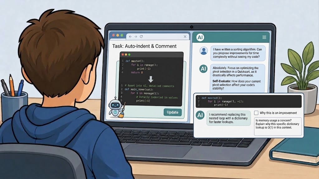
Fig 1. Image generated with ChatGPTGemini (GPT3.6 Image 2)Thinking), AugustSeptember 27,8, 2026.

Content

MathematicalProgramming modelseducation is changing in a context where AI systems can generate, explain, and computerreview simulationscode. While these tools offer new opportunities for learning, they also introduce an important educational challenge: students need sufficient programming knowledge to evaluate whether an AI-generated suggestion is correct, efficient, or even relevant to the task at hand. Without a basic understanding of programming concepts, students may accept incorrect solutions, overlook errors, or fail to recognize better alternatives. For this reason, learning programming fundamentals remains essential, even when AI tools are especiallyavailable.

valuable

In toolsintroductory programming courses, AI should be positioned as a learning support tool rather than as a substitute programmer. Students can use AI effectively for repetitive or low-level tasks that do not reduce the cognitive effort involved in ecology, because they can express highly complex systems through mathematical equations. This makes it possiblelearning to runprogram. experimentsExamples ininclude silicoformatting and testindenting hypothesescode, generating documentation comments, explaining error messages, summarizing syntax rules, or helping students understand the purpose of specific programming constructs. These uses allow students to focus their attention on the underlying logic, algorithms, and problem-solving processes that are central to programming competence.

Another productive use of AI is code review. Instead of asking an AI model into situations wherewrite a realsolution, experimentstudents wouldcan bewrite tootheir costly,own toocode slow, ethically difficult, or outright dangerous. Manipulating a real predator population, for instance, is rarely an option. At the same time, every model is necessarily a simplification of reality,first and thisthen is exactly where its weaknesses lie: real ecosystems are far more complex than any model can fully capture.

The Lotka–Volterra model is a classic example of such a simplification applied to predator–prey dynamics. It represents the system using two state variables (the prey and predator population sizes) and four parameters (the prey’s intrinsic growth rate, the predation-rate coefficient, the predator’s reproduction rate per prey consumed, and the predator’s mortality rate). Under its idealized assumptions,ask the model predictsto sustained,identify periodicpotential oscillationsimprovements. inThe whichAI changesmight insuggest clearer variable names, better code organization, reduced redundancy, improved readability, or alternative approaches that the predatorstudent populationcan lagevaluate behindindependently. thoseThis intransforms the preyAI population. This behavior arises frominto a feedback loop:partner, allowing students to compare their own reasoning with external suggestions and assess the strengths and weaknesses of their solutions.

However, AI-generated feedback should not be accepted uncritically. Models may recommend changes that are unnecessary, inefficient, or based on incorrect assumptions about the code's purpose. A central goal of this lesson is therefore to develop students' ability to critically evaluate AI suggestions. Students will learn to ask an AI model not only what improvements it proposes, but also why it considers those changes beneficial. By comparing the model's reasoning to established programming principles, students can judge whether the proposed optimization genuinely improves the code or merely represents a different design choice.

This lesson treats AI as thea preytool populationthat increases,supports morereflection, foodself-assessment, becomesand availablecode quality improvement rather than code generation. Students practice writing their own programs, using AI to predators,perform allowingsupportive tasks, requesting feedback on their work, and critically analyzing the predator population to grow. Increased predation then causes the prey population to decline, which reduces the predators’ food supply and leads to a decline in the predator population. With fewer predators, the prey population can recover, and the cycle begins again.

To produce this clean cycle, the model makes several strong assumptions. It is deterministic (the same starting values always produce exactly the same curve); it is a closed two-species system that excludes every abiotic factor (temperature, precipitation, season) and every other biotic factor (food plants for the prey, a third species, disease); and it makes each population's growth depend on nothing except the sizequality of the otherresponses population.they receive. The ultimate objective is to help students become both better programmers and more informed users of AI systems.

Real populations rarely meet these assumptions. Births, deaths and encounters are subject to chance, and a stochastic (randomised) version of the same model tends to drift away from the clean cycle and can even collapse (e.g. the predator population dying out) in cases where the deterministic version predicts stable oscillation. Likewise, adding just a single missing factor (e.g. a temperature-dependent growth rate, or a limit on the prey's own food supply) is often enough to break the clean two-variable cycle. This is not a flaw to hide from students, it is the central Nature-of-Science lesson of the activity. A model can be genuinely useful, while still being a deliberately narrow approximation of reality and using it well means knowing exactly which factors it leaves out. In this lesson's main activity, students discover this for themselves by trying to add exactly these kinds of factors.

Lesson plan

Phase	Time	Activity
Introduction	8 min	The teachers shows an unlabelled graph of a real predator–prey data series (e.g. lynx/hare); students describe the pattern and form first hypotheses.
Input	12 min	The teacher introduces the model’s variables and parameters using a simple diagram (no differential equations needed).
Exploration	15 min	Students test their hypotheses in pairs on a ready-made HTML simulation and record their observations.
Adaptation	35 min	In pairs, students work through 2–3 rounds of predict → prompt → test → diagnose (guiding questions below), each time asking the LLM to add one more layer of ecological realism to the simulation (a limit on the prey's food supply, a second species, a seasonal/abiotic factor) until the clean two-variable cycle visibly breaks down.
Reflection	20 min	Whole-class discussion, guided by questions such as: At which round did the simulation stop producing a clean, repeating cycle? What does the original model deliberately leave out, and why? What makes it a useful simplification rather than simply a wrong one?

Guiding questions: layering complexity

Pairs work through as many of the following rounds as time allows in the 35 minutes (most manage two; the third is an extension for early finishers). Each round follows the same four-step cycle:

1. Round 1 — limit the prey's food supply (a carrying capacity):
   • Predict: Before you start prompting, aks yourself: what do you expect to happen to the cycle if the prey's growth slows down once the population gets large, instead of growing without limit? Sketch the curve you expect.
   • Prompt: Ask the AI to add a maximum sustainable prey population to the simulation, and to explain in its own words how it changed the growth equation to do this.
   • Test & compare: Run the new simulation with the same starting values as before. Compare the previous simulation with the new one: how did the variables change? Why is that?
   • Diagnose: Which assumption of the original model (unlimited food for the prey) did you just remove? Is this factor biotic or abiotic?
2. Round 2 — add another (biotic or abiotic) factor:
   • Predict: If a third species now competes with the prey for food, or preys on it as well, or if prey growth now depends on temperature what do you expect this to do to the original two-species cycle?
   • Prompt: Choose another factor and write a prompt asking the AI to add it as a new variable linked to the existing ones — specify exactly how it should interact with the prey or predator population.
   • Test & compare: Observe the simulation over several cycles. Does the original two-species rhythm survive, get distorted, or disappear?
   • Diagnose: The original model assumed each population depends only on the other. Is that still true after this round? What real ecological relationship does your new factor represent.
3. Optional round 3 — introduce randomness:
   • Predict: If one parameter (e.g. the predation rate) is no longer fixed but drawn randomly within a range at each time step, what do you expect for the long-term stability of the populations?
   • Prompt: Ask the AI to replace one constant parameter with a randomised value and to keep track of whether either population reaches zero.
   • Test & compare: Run the simulation several times with the same settings. Do you get the same result every time? Does either population ever collapse?
   • Diagnose: Why can the same “average” parameter values sometimes lead to extinction here, when the deterministic model never predicted that?

Closing question (for the Reflect phase): At which round did the simulation stop producing a clean, repeating cycle — and what does that tell you about how many real-world factors the original Lotka–Volterra model has to leave out in order to stay solvable and easy to interpret?

Materials

• One laptop per student pair, with a browser
• Access to an LLM chat interface via the internet, or a locally installed model if internet access is restricted at school
• Ready-made HTML predator–prey simulation (single file, sliders for selected parameters)
• A short prompting / worksheet template for the “layering complexity” rounds (predict → prompt → test → diagnose)
• Guiding questions for the exploration phase and the Nature-of-Science reflection (model purpose vs. model limits)